Wellbore Stability and Horizontal Stresses
“I paid to send the entire crew to a 5-day ERD practices class, had an engineering study done, and put ERD hands on my rig — and I still got stuck!”
Maybe you have another problem, one that conventional ERD companies don’t address…
HXR Drilling Services’ Geomechanics Division provides solutions for wellbore stability uncertainties. Instability issues can be avoided by developing a geomechanical model based on data collected from regional offset wells using JewelSuite™, a 1D and 3D subsurface modeling platform. JewelSuite™ modular software platform is made up of PressCheck™ and WellCheck™, and is commonly used with another stress modeling program, call SFIB™. One essential function of the geomechanical model is to define stresses to avoid instability issues. This allows drilling personnel to develop a sound drill plan with the best mud weights, drill trajectory, and casing design.
This article describes how the horizontal stress aspect plays a critical part in wellbore instability. The stress data can be shown as a 1D graph, which provide data points at multiple depths and is characterized as a single 1D curve.
Before horizontal stresses can be defined there is required data that must be available and/or calculated. HXR’s personnel calculate the effective stress and further calculates the maximum and minimum horizontal stress downhole, as well as, the azimuth of maximum horizontal stress. The required data is comprised of lithology information, rock properties/UCS, overburden stress, and interpreted pore pressure. LOT and RFT values are helpful calibration points used to develop custom trend lines. The custom trend line interpolates the points to calculate and calibrate the horizontal stresses for the effective stress curve. The Horizontal Stress Model gives unitless effective-stress-ratio points, as seen in Figure 1a and 1b.
JewelSuite™ PressCheck™ and WellCheck™ software provides three methods to analyze the horizontal stresses termed Effective Stress Method, Stress Contrast, and SHmax Equilibrium Ratio. Each method provides different information related to the stresses.
Effective Stress Method
The Effective Stress Method calculates the maximum and minimum horizontal stresses from overburden stress, pore pressure and Shmin and SHmax effective stress calibration points. The equations used in this method are:
Maximum Effective Stress Ratio= (SHmax-PP) / (Sv-PP)
Minimum Effective Stress Ratio= (Shmin-PP) / (Sv-PP)
Where Sv is the vertical stress or overburden stress, PP is pore pressure, and SHmax and Shmin are maximum horizontal stress and minimum horizontal stress respectively. Additional information relating to stress state, such as LOT/FIT and RFTs, are plotted on the track along within the Horizontal Stress Model View as calibration points to generate interpreted trend lines. The Horizontal Stress View displays tracks for the interpreted pore pressure and overburden stress curves, as well as the calibration points for Shmin and SHmax.
Horizontal Stress Modeling View
Figure 1a and 1b. Horizontal Stress Modeling Panel with horizontal stresses (MPa). 1a. Overburden gradient, calibration points LOT’s and RFT’s, custom trends, and effective stresses displayed. 1b. SHmax and Shmin final values giving in MPa.
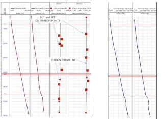
Figures 1a and 1b
Calculating Horizontal Stress from Existing Logs Using the Stress Contract Method
No Tectonic Strain, Isotropic Tectonic Strain, Tectonic Strain
The Stress Contrast method derives Shmin and SHmax stresses from existing logs. There are three types of equations used that are dependent on the regional geology known as No Tectonic Strain, Isotropic Tectonic Strain, and Tectonic Strain (Figure 2).
No Tectonic Strain
The No Tectonic Strain method is based on bilateral constraint that uses an equation developed by Eaton, where ϑ is equal to stress.
Shmin = (ϑ/1 – ϑ) (Sv−PP) + PP
Isotropic Tectonic Strain
Isotropic Tectonic Strain considers the Biot coefficient equal to 1. The first half of the equation represents the horizontal stress for a relaxed homogenous, laterally extended half space (uniaxial strain) after applying an infinite load instantaneously. The last term of the model corresponds to the tectonic strain. Where Eε is Young’s modulus in Pascals.
Shmin = (ϑ/1 – ϑ) (Sv−PP) + PP + (1 + ϑ / 1- ϑ2) Eε
Tectonic Strain
Tectonic Strain is the same equation as the Isotropic Tectonic Strain equation above but with a Biot coefficient different from 1.
Shmin = (ϑ/*other Biot- ϑ) (Sv−PP) + PP + (*other Biot + ϑ / *other Biot- ϑ2) Eε
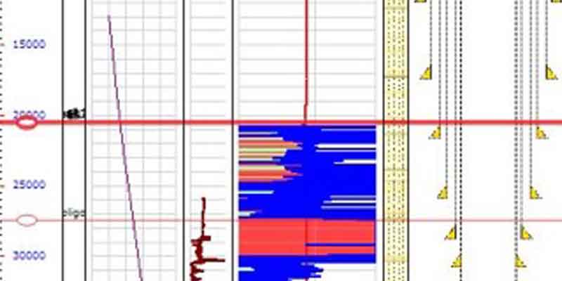
Stress Contrast View
Figure 2. Overburden stress is in gold, interpreted pore pressure in red, and both maximum and minimum stresses are shown in blue. Additionally, the curves for static Poisson’s Ratio and Static Young’s Modulus are shown on the far left track.

Figure 2
Calculating Maximum Horizontal Stress from the Equilibrium Ratio Method
The SHmax/Equilibrium method sets the SHmax parameter on one of the three stress states defined by frictional faulting theory. The frictional fault theory is a hypothetical theory stating 2 of 3 principle stresses need to be parallel with the surface of the earth (Figure 3).
Principle Stress Directions for the Frictional Faulting Theory
Figure 3. Visual Representation of Principle Stress Directions for the Frictional Faulting Theory

Figure 3
Normal faulting stress regime requires that SHmax is the intermediate principal stress magnitude, Shmin is the least principal stress, and Sv is the maximum principal stress typically seen as Sv > SHmax > Shmin.
Strike-slip faulting and reverse faulting regimes require that SHmax is the maximum principal stress magnitude. Strike-slip stress are typically seen in literature as SHmax > Sv > Shmin, whereas reverse faulting is shown as SHmax > Shmin > Sv. Within JewelSuite™ WellCheck™, the curves in the SHmax/Equilibrium Ratio View shows the results of the calculation in terms of normal and EMW’s (Figure 4).
SHmax / Equilibrium Ratio View
Figure 4. In this figure, one track shows the curves as pressure (MPa) and the second is equivalent mud weight (EMW)

Figure 4
Mud Weight Predicted and Checked
After the stress data is calculated the critical mud pressures that contribute to wellbore collapse and breakout values now can be calculated and proposed mud weights can be checked. Running the proposed mud weights within the model provides predictions for wellbore collapse and breakout at any given depth.
Mud weights can be evaluated for a target well to model wellbore failure along the well trajectory, which is dependent on the calculated stress state and rock properties. The Check Mud Weight View serves as a representation of the degree of breakout (BO), which is also referred to as the failed zone. The Check Mud Weight view displays the mud weight log in the first track and the break out width (BOW) and critical break out width (CBOW) in the second track (Figure 5).
Check Mud Weight View
Figure 5. The allowable weight is in blue, breakout width below critical breakout limit is green, and the exceedance of the limit is in red. In this particular model, the mud weight chosen for this offset well was a too high and viewing the caliper data versus the breakout (red circle) there appears to be problems at the bottom of the hole, perhaps a washout.

Figure 5
HXR Drilling Services’ Geomechanics Division provides solutions by producing a geomechanical model that defines stable wellbore trajectories and determines optimal mud weights based on stresses within the subsurface. This article covered stresses and pore pressures downhole to demonstrate the assessments that HXR Drilling Services Geomechanics has to offer clients, see Figure 5. The casing and mud weights can be designed and modified based on several different wellbore trajectories to find the most cost efficient plan.
Talk to HXR when you’re ready to plan your next horizontal or ERD development.
Posted on: February 4th, 2016
Filed under: Blog, Extended Reach Drilling, Geomechanics, Software Solutions, Wellbore Stability